Week 09: Disjoint Sets and Minimum Spanning Trees (Lab)

Bingjie Xu

2026-03-05

Intro

Learning Objectives

By the end of this lab session, you should be able to:

1. Implement disjoint set (union-find) data structures in C++.
2. Implement Minimum Spanning Tree (MST) algorithms (Kruskal’s and Prim’s) in C++.
3. Apply MST algorithms to solve real-world connectivity problems.

Overview of Lab Activities

This lab consists of three main activities:

1. MCQs (10 marks)
   • Two matching exercises to understand Kruskal’s and Prim’s MST
   • Complete xSITe quizzes.
2. Minimum Cost Spanning Tree (20 marks)
   • Implement Kruskal’s or Prim’s algorithm in C++ to find the minimum cost to connect all points in a 2D plane.
   • Submit your C++ implementation via Gradescope.
3. Real-world Application: Simple Image Segmentation (30 marks)
   • Implement an MST-based algorithm in C++ to compute the minimum total “dissimilarity” cost for a small grayscale image.
   • Use this MST to reason about how the image can be segmented into background and foreground.
   • Submit your C++ implementation via Gradescope.

What is a Minimum Spanning Tree?

A Minimum Spanning Tree (MST) of a connected, undirected, weighted graph is a spanning tree with the minimum possible total edge weight.

Key properties:

• Connects all vertices in the graph
• Contains no cycles
• Has exactly \(|V| - 1\) edges
• Minimizes the total edge weight

Use Cases of MST

Minimum Spanning Trees have numerous real-world applications:

• Network Design: Designing computer networks, telephone networks, or electrical grids with minimum cost
• Transportation Planning: Connecting cities with roads or railways at minimum cost
• Circuit Design: Minimizing wire length in circuit board design
• Image Segmentation: Segmenting images by modelling pixels as nodes and minimizing the total dissimilarity between connected pixels.

Activity 1: Multiple Choice Questions

Matching Exercise: MST Edge Selection Order

Given the weighted graph below, determine the order in which edges are selected when applying Kruskal’s algorithm and Prim’s algorithm (starting from vertex a).

Instructions

• For Kruskal’s algorithm: List the edges in the order they are added to the MST (by weight, breaking ties alphabetically).
• For Prim’s algorithm: List the edges in the order they are added to the MST when starting from vertex a.

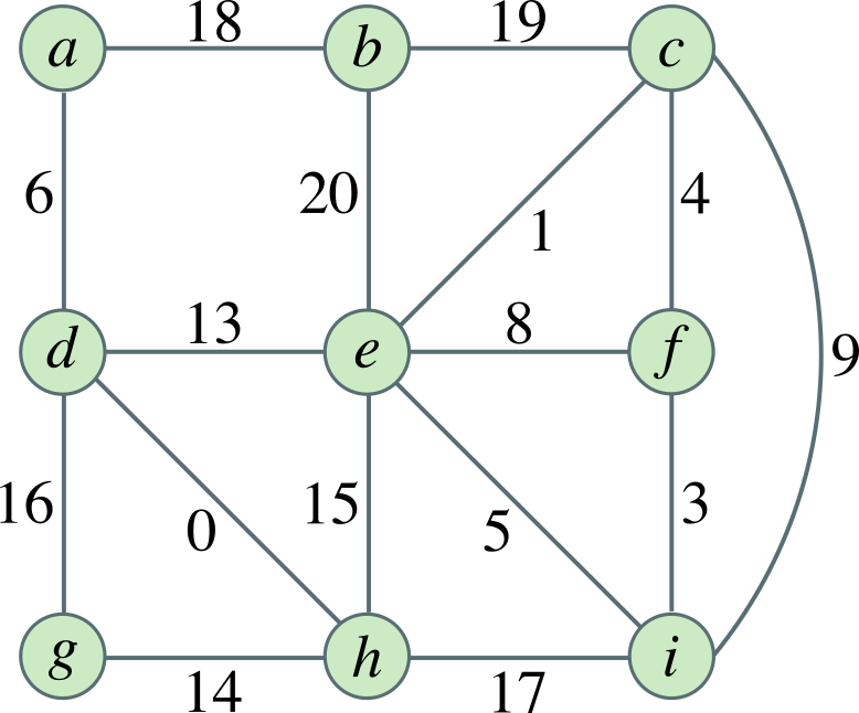
Submission (xSITe Quizzes, 10 marks). Matching the order of edges for both algorithms from xSITe Quiz “Week 09 Lab Exercise 1”.

Activity 2: Minimum Cost Spanning Tree

Problem Description

You are given an array of points where points[i] = \([x_i, y_i]\) represents a point on a 2D plane. Your task is to find the minimum cost to make all points connected, where the cost of connecting two points \([x_i, y_i]\) and \([x_j, y_j]\) is the Manhattan distance between them: \(|x_i - x_j| + |y_i - y_j|\).

This is essentially finding the Minimum Spanning Tree (MST) of a complete undirected graph where:

• Each point is a vertex
• The weight of an edge between two points is their Manhattan distance

Problem Description (Cont.)

Constraints

• \(1 \leq n \leq 1000\), where \(n\) is the number of points
• \(-10^6 \leq x_i, y_i \leq 10^6\)
• All points are distinct

Exercise

1. Download min_cost.zip from xSITe. The file min_cost.cpp contains a stub for function

   int minCost(vector<vector<int>> &points);

2. Implement minCost using Kruskal’s or Prim’s algorithm to find the MST.

3. Build a complete graph where each edge weight is the Manhattan distance between two points.

4. Use appropriate data structure (Disjoint Sets or min-heap) to efficiently select the minimum-weight edge at each step.

5. Make and test your implementation locally using the provided test.txt.

Submission (Gradescope, 20 marks). Submit your completed min_cost.cpp and min_cost.h to the “Week 09 Lab Exercise 2” assignment on Gradescope.

Key Points

• Calculate Manhattan distance: \(|x_i - x_j| + |y_i - y_j|\)

• Prim’s Algorithm approach:

  • Start with an arbitrary vertex
  • At each step, add the minimum-weight edge that connects a vertex in the MST to a vertex outside the MST (avoid cycle)
  • Use a priority queue (min-heap) to efficiently find the minimum-weight edge
  • Maintain a visited array to track vertices already in the MST

• Kruskal’s Algorithm approach:

  • Sort edges by weight in ascending order
  • Use Union-Find (Disjoint Set) data structure to detect cycles by checking the representative
  • Add edges in order if they don’t create cycles
  • Stop when \(|V| - 1\) edges have been added

Activity 3: Simple Image Segmentation with MST

Problem Description

You are given a small grayscale image. Each pixel can be modelled as a vertex in a graph. Two neighbouring pixels (up, down, left, right) are connected by an edge whose weight is the absolute difference in pixel intensity between the two pixels (their dissimilarity).

An MST on this graph connects all pixels while minimizing the total dissimilarity between neighbouring pixels. If we cut (remove) the largest-weight edges in the MST, the image is split into regions (segments) of similar intensity.

Key idea: MST ensures that within each segment, neighbouring pixels are as similar as possible, and segmentation is achieved by removing the largest dissimilarities (heaviest edges) in the tree.

Problem Description (Cont.)

Consider the following \(3 \times 3\) grayscale image, where each number is a pixel intensity:

1. Graph construction: Treat pixels as vertices, connect 4-neighbours, weight = absolute intensity difference.
2. MST by hand:
   • List all edges with weights for the 3×3 image.
   • Use Kruskal’s algorithm by hand (Prim’s is also fine): sort edges by weight, add them one by one, skipping cycles, until all pixels are connected.
3. Segmentation by cutting the MST:
   • From your MST, identify the largest-weight edge(s) (i.e., between 12 and 201, or 13 and 202).
   • Cutting these splits the MST into two components: top 2×3 block (background) vs bottom row (foreground).

Problem Description (Cont.)

Consider the following \(3 \times 3\) grayscale image, where each number is a pixel intensity:

Below is one of the valid MSTs:

Exercise

1. Download: Get image_segmentation.zip from xSITe. The starter file image_segmentation.cpp contains the stub:

   int imageMSTCost(int rows, int cols, const vector<int> &pixels);

2. Input format:

   • First line: rows cols (image height and width)
   • Next rows lines: each line has cols integer pixel intensities in \([0, 255]\) (grayscale values)

3. Output format: You do NOT need to actually output the segmentation. Just compute the MST total “dissimilarity” cost of the image.

4. Implementation hints:

   • Map \((row, col)\) to a 1D index: idx = row * cols + col
   • Only add edges right and down (to avoid duplicates), but still model 4-neighbour connectivity

Submission (Gradescope, 30 marks). Upload completed image_segmentation.cpp file to Gradescope “Week 09 Lab Exercise 3”.

Conclusion

Wrap-up

By the end of this lab you should be able to:

1. Understand the concept of Minimum Spanning Tree (MST)
2. Use appropriate data structures to implement Kruskal’s or Prim’s algorithm to find MST
3. Apply MST algorithms to solve connectivity problems with minimum cost

Outlook

This lab introduced Minimum Spanning Trees as a fundamental graph algorithm. The remaining weeks cover:

Single-Source Shortest Paths

Dijkstra’s and Bellman-Ford algorithms for finding shortest paths from a source vertex

Dynamic Programming and Greedy Algorithms

Versatile optimization techniques for solving complex problems