Learning Objectives
By the end of this lecture, you should be able to:
- Define key features of an algorithm, including input size and basic steps.
- Express an algorithm’s running time as a function \(T(n)\).
- Use asymptotic notation (\(O\), \(\Omega\), \(\Theta\)) to describe and compare running times.
- Derive the asymptotic running times of non-recursive algorithms by counting basic steps.
- Recognize key properties of divide-and-conquer algorithms.
- Solve divide-and-conquer recurrences using recursion trees and the Master Theorem.
From Week 01 to Week 02
Last week, we stated the following objectives for studying data structures and algorithms:
Is the computational procedure correct?
Does it always terminate?
Given a particular data structure as input, how much
- time does the procedure take?
- memory does the procedure use?
We addressed Questions 1 and 2 in Week 01. Today, we focus on Question 3a: running times.
What Do We Mean by “Running Time”?
In everyday language, an algorithm’s running time is the time on a clock (e.g., seconds).
In this course, we usually do not measure seconds directly, because they depend on:
- the computer and its CPU,
- the programming language and compiler,
- and many implementation details.
Instead, we use a machine-independent model:
The running time \(\boldsymbol{T(n)}\) of an algorithm is the number of basic steps (e.g., comparisons, assignments, and arithmetic operations) it performs on an input of size \(n\) (e.g., the number of keys to sort).
Later, we will compare algorithms by how \(T(n)\) grows as \(\boldsymbol{n}\) increases.
What Counts as a “Basic Step”?
To make \(T(n)\) meaningful, we use a simple cost model:
A basic step is either
- one operation on a value with a fixed number of bits (e.g., a 32-bit integer or a 64-bit floating-point number), or
- one access to a single array element \(A[i]\), given the index \(i\).
We assume that each basic step takes at most a constant amount of time, regardless of the input size \(n\).
This model simplifies reality, but it lets us compare algorithms without depending on a particular CPU, compiler, or programming language.
Running Times of Non-Recursive Algorithms
For non-recursive algorithms, we will derive \(T(n)\) as follows:
- Specify what the input size \(n\) measures for this problem.
- Count how many basic steps are executed, as a function of \(n\).
- Sum the counts to obtain \(T(n)\).
Rule of thumb: Nested loops usually multiply counts.
For example, if an outer loop runs \(n\) times and the inner loop runs \(n\) times for each outer iteration, then the inner-loop body executes \(n^2\) times:
Input: array a with n elements

for i ← 0 .. n - 1
    for j ← 0 .. n - 1
        a[i] ← a[i] + 1
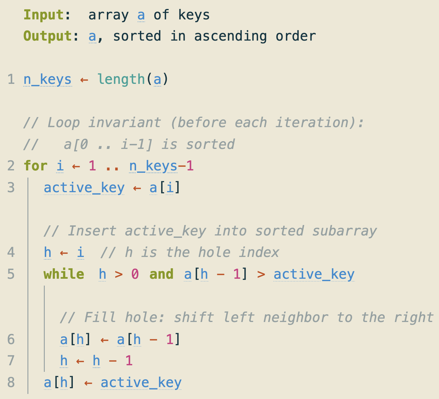
Example: Insertion Sort
![]()
The highlighted basic steps are not the only ones, but they are enough to characterize the running time.
Insertion Sort on an Array Sorted in Ascending Order
Open https://apps.michael-gastner.com/insertion-sort/ and choose ascending-order input from the example dropdown. You can edit the input by typing in the text box. Increase the input size (try 5, 10, and 20 keys) and observe how the Final counts of the following metrics change:
- Left-boundary checks
- Comparisons with active key
- Right shifts
- Insertions
Do the observations match your expectations?
Insertion Sort on an Array Sorted in Descending Order
Open https://apps.michael-gastner.com/insertion-sort/ again. This time, choose descending-order input from the example dropdown. Again, increase the input size (try 5, 10, and 20 keys) and observe how the Final counts of the following metrics change:
- Left-boundary checks
- Comparisons with active key
- Right shifts
- Insertions
Which metric grows fastest as \(n\) increases?
Focus on the Dominant Growth Trend
On the previous slides, we counted basic steps for insertion sort and observed two different growth patterns:
- If the input is in ascending order, the step counts grow roughly in proportion to \(n\).
- If it is in descending order, they grow approximately in proportion to \(n^2\).
When we compare algorithms, we care most about what happens as the input gets large. In that regime, the dominant growth trend matters more than small details such as the “\(+1\)” effect in the left-boundary checks.
Asymptotic Notations: \(O\), \(\Omega\), and \(\Theta\)
To describe the dominant growth trend of a running-time function \(T(n)\) for large \(n\), we compare it to a simpler function \(g(n)\). We ask whether a constant multiple of \(g(n)\) provides an upper bound, a lower bound, or both for \(T(n)\) once \(n\) is sufficiently large. We will make this notion mathematically precise on the following slides.
| \(O(g(n))\) |
Big O |
Upper |
| \(\Omega(g(n))\) |
Big Omega |
Lower |
| \(\Theta(g(n))\) |
Theta |
Tight (upper and lower) |
For instance, the upcoming definitions allow us to state the insertion-sort results as:
- Best case (ascending order): \(\Theta(n)\)
- Worst case (descending order): \(\Theta(n^2)\)
\(O\)-Notation: Definition
The \(O\)-notation describes the upper bound of a function’s growth rate.
Let \(g(n)\) be a function such that \(g(n) \ge 0\) for all \(n \ge n_0\) (for some \(n_0\)). Then \(O(g(n))\) denotes the set of functions
\[\begin{equation*}
\begin{aligned}
O(g(n)) = \{f(n) :\ & \text{there exist positive constants } c \text{ and } n_0 \text{ such that }\\
& |f(n)| \leq c g(n) \text{ for all } n \geq n_0\}.
\end{aligned}
\end{equation*}\]
\(O\)-Notation: Example
Insertion sort has a worst-case running time of the form \(T(n) = qn^2 + rn + s\) for some constants \(q\neq 0\), \(r\), and \(s\).
Choose \(c = |q| + |r| + |s|\) and \(n_0 = 1\). Then, for all \(n \ge n_0\),
\[\begin{equation*}
\begin{aligned}
|T(n)|
&= |qn^2 + rn + s| \\
&\le |q| n^2 + |r| n + |s| \\
&\le |q| n^2 + |r| n^2 + |s| n^2 \\
&= (|q| + |r| + |s|) n^2 = c n^2,
\end{aligned}
\end{equation*}\] where the first inequality follows from the triangle inequality, and the second inequality holds because \(n \ge 1\) implies \(n \le n^2\).
Hence, \(T(n) \in O(n^2)\).
\(\Omega\)-Notation: Definition
The \(\Omega\)-notation describes the lower bound of a function’s growth rate.
Let \(g(n)\) be a function such that \(g(n) \ge 0\) for all \(n \ge n_0\) (for some \(n_0\)). Then \(\Omega(g(n))\) denotes the set of functions
\[\begin{equation*}
\begin{aligned}
\Omega(g(n)) = \{f(n) :\ & \text{there exist positive constants } c \text{ and } n_0 \text{ such that }\\
& |f(n)| \geq c g(n) \text{ for all } n \geq n_0\}.
\end{aligned}
\end{equation*}\]
\(\Omega\)-Notation: Example
Consider again the insertion sort’s worst-case running time \(T(n) = qn^2 + rn + s\) with \(q \neq 0\). Choose \(c = |q|/4\) and \(n_0 = \max \left(1,\ 2|r/q|,\ 2\sqrt{|s/q|}\right).\) Then, for all \(n \ge n_0\), we have \(|r|n \le \frac{|q|}{2}n^2\) and \(|s| \le \frac{|q|}{4}n^2\). Hence, by the reverse triangle inequality,
\[\begin{equation*}
\begin{aligned}
|T(n)|
&= |qn^2 + rn + s| \\
&\ge |q|n^2 - |r|n - |s| \\
&\ge |q|n^2 - \frac{|q|}{2}n^2 - \frac{|q|}{4}n^2 \\
&= \frac{|q|}{4}n^2 = c n^2.
\end{aligned}
\end{equation*}\]
Therefore, \(T(n) \in \Omega(n^2)\).
\(\Theta\)-Notation: Definition
The \(\Theta\)-notation describes the tight bound of a function’s growth rate.
Let \(g(n)\) be a function such that \(g(n) \ge 0\) for all \(n \ge n_0\) (for some \(n_0\)). Then \(\Theta(g(n))\) denotes the set of functions
\[\begin{equation*}
\begin{aligned}
\Theta(g(n)) = \{f(n) :\ & \text{there exist positive constants } c_1, c_2, \text{ and } n_0 \text{ such that }\\
& c_1 g(n) \leq |f(n)| \leq c_2 g(n) \text{ for all } n \geq n_0\}.
\end{aligned}
\end{equation*}\]
Instead of writing \(f(n) \in \Theta(g(n))\), it is common to use the shorthand \(f(n) = \Theta(g(n))\). The same convention applies to \(O\) and \(\Omega\) notations.
Relationship Between \(\Theta\), \(O\), and \(\Omega\)
For any two functions \(f(n)\) and \(g(n)\), the following equivalence holds:
\[\begin{equation*}
f(n) \in \Theta(g(n)) \quad \text{if and only if} \quad f(n) \in O(g(n)) \ \text{and} \ f(n) \in \Omega(g(n)).
\end{equation*}\]
For instance, we have shown that the worst-case running time of insertion sort satisfies \(T(n) \in O(n^2)\) and \(T(n) \in \Omega(n^2)\). Therefore, \(T(n) \in \Theta(n^2)\).
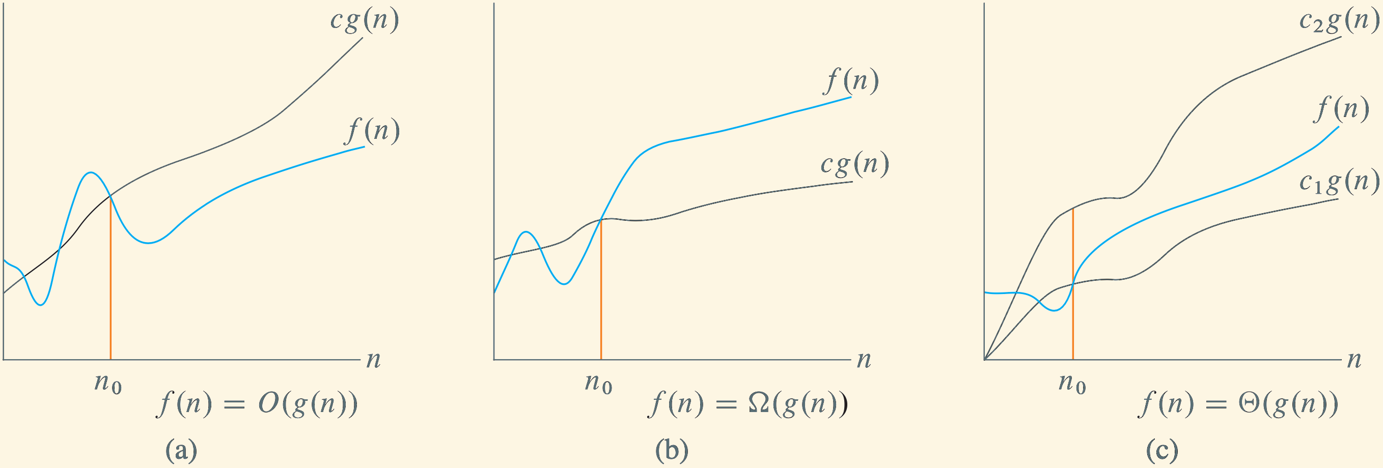
Illustration of Asymptotic Notations
Figure 3.2 from Cormen et al. (2022):
![]()
State the Tightest and Simplest Known Bound
As a matter of style:
- If you can prove that a function is \(\Theta(g(n))\), state \(\Theta(g(n))\); do not use \(O\) or \(\Omega\) instead.
- Otherwise, state the tightest bounds you can justify. For example, any function that is \(O(n^2)\) is also \(O(n^3)\), but \(O(n^2)\) is more informative because it provides a tighter upper bound.
- Use the simplest functions possible. For instance, if a function is \(\Theta(n^2)\), it is also \(\Theta(9n^2 - 2n)\), but \(\Theta(n^2)\) is clearer and more concise.
- When we write \(f(n) = O(g(n))\), the “\(=\)” sign is shorthand for set membership; do not treat it as algebraic equality.
Common Growth Rates (From Smallest to Largest)
For sufficiently large \(n\), the following functions grow in this order:
- \(1\) (constant)
- \(\log n\) (logarithmic). The base of \(\log n\) is irrelevant in asymptotic notation because changing the base only introduces a constant factor.
- \((\log n)^k\) for \(k > 0\) (polylogarithmic)
- \(n^z\) for \(0 < z < 1\) (sublinear power law, e.g., \(\sqrt{n}\))
- \(n\) (linear)
- \(n \log n\) (linearithmic)
- \(n^k\) for \(k > 1\) (polynomial; includes \(n^2, n^3, \ldots\))
- \(a^n\) for \(a > 1\) (exponential; e.g., \(2^n\))
- \(n!\) (factorial)
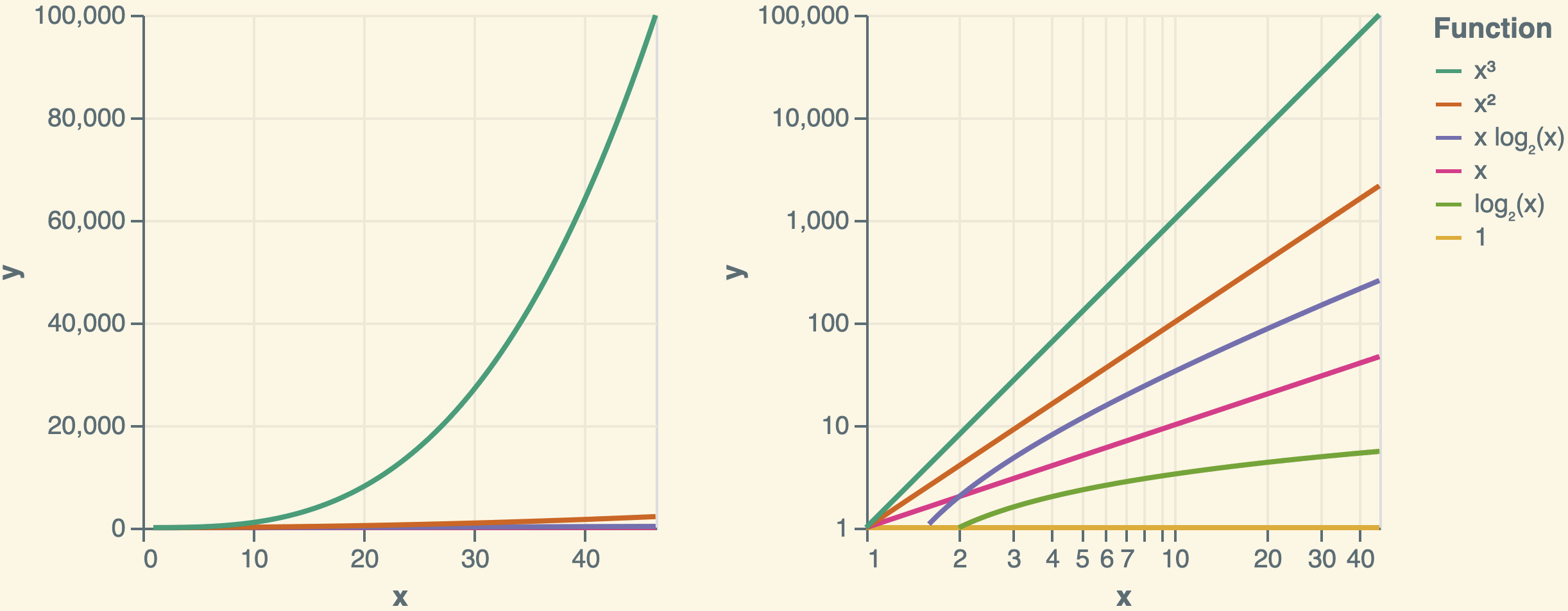
Plots of Common Functions
The plots below illustrate functions commonly encountered in running-time analysis. The left plot uses linear scales for both the \(x\)-axis and \(y\)-axis, whereas the right plot employs logarithmic scales.
![]()
Quiz: Ordering by Asymptotic Growth Rates
Rank the following functions of \(n\) by order of growth; that is, find an arrangement \((g_1, g_2, g_3, g_4)\) of the functions from slowest-growing to fastest-growing:
- \(\log n\)
- \(n^2\)
- \(n \log n\)
- \(n\)
Divide-and-Conquer Algorithms
In Week 01, we defined a recursive algorithm as one that calls itself.
So far, we have derived the running time of a non-recursive algorithm: insertion sort. As we saw in this example, non-recursive algorithms usually require counting how often each operation is executed.
For recursive algorithms, different techniques are required. Divide-and-conquer algorithms are a prominent class of recursive algorithms, and several methods exist for analyzing their running times.
A divide-and-conquer algorithm typically consists of three key steps, listed on the following slide.
Three Steps of Divide-and-Conquer Algorithms
- Divide: Partition the problem into one or more subproblems, each representing a smaller instance of the same problem.
- Conquer: Solve the subproblems recursively until they reach a base case that can be solved directly.
- Combine: Integrate the solutions of the subproblems to obtain a solution to the original problem.
Merge Sort: An Example of Divide-and-Conquer
You implemented merge sort in Week 01. It is a paradigmatic example of a divide-and-conquer algorithm:
![]()
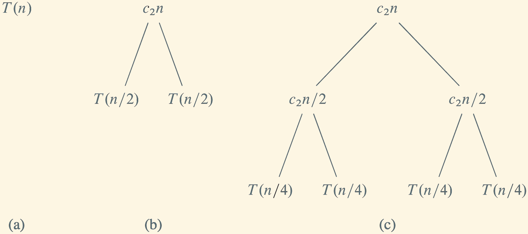
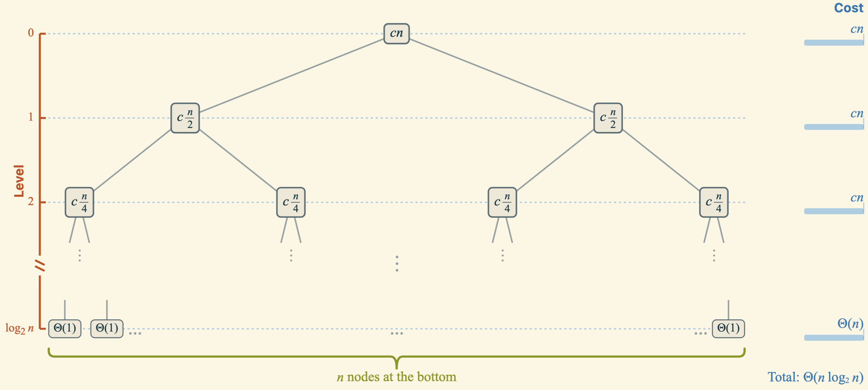
Recurrence Relation for Merge Sort’s Running Time
Summarizing the time required by the divide, conquer, and combine steps, we obtain the following recurrence relation for merge sort’s running time. For simplicity, we assume that the input size \(n\) is a power of two:
\[
T(n) = 2T(n/2) + \Theta(n).
\tag{1}\]
Note that Equation 1 implies that there exist constants \(c_1, c_2 > 0\) such that
\[\begin{equation*}
c_1 n \leq |T(n) - 2 T(n/2)| \leq c_2 n
\end{equation*}\]
for all sufficiently large \(n\).
Next, we will represent the recurrence relation as a tree and derive \(T(n)\) from it.
Master Theorem
Although recursion trees help build intuition, they do not by themselves provide a mathematically rigorous method for solving recurrences. The Master Theorem provides an alternative technique with mathematical guarantees.
Let \(a \ge 1\) and \(b > 1\) be constants, and let \(f(n)\) be a function with \(f(n) \ge 0\) for all sufficiently large \(n\). Consider recurrences of the form \(T(n) = a\,T\left(\frac{n}{b}\right) + f(n)\) for values of \(n\) for which the recurrence is defined (e.g., \(n=b^k\)). Let \(p = \log_b a\).
- If \(f(n) \in O\bigl(n^{p-\varepsilon}\bigr)\) for some \(\varepsilon > 0\), then \(T(n) \in \Theta\bigl(n^p\bigr)\).
- If there exists \(k \ge 0\) such that \(f(n) \in \Theta\bigl(n^p \log^k n \bigr)\), then \(T(n) \in \Theta\bigl(n^p \log^{k+1} n\bigr)\).
- If \(f(n) \in \Omega\bigl(n^{p+\varepsilon}\bigr)\) for some \(\varepsilon > 0\) and there exist constants \(c < 1\) and \(n_0\) such that for all \(n \ge n_0\) we have \(a\,f\left(\frac{n}{b}\right) \le c\,f(n)\), then \(T(n) \in \Theta\bigl(f(n)\bigr)\).
Applying the Master Theorem to Merge Sort
Recall the merge sort recurrence: \(T(n) = 2 T(n/2) + \Theta(n)\), so \(a = 2\), \(b = 2\), and \(f(n) = n\).
First, we compute \(p = \log_b a = \log_2 2 = 1\). Case 2 of the Master Theorem applies with \(k=0\).
Therefore, the total running time is \(T(n) = \Theta\bigl(n^1 \log^{0+1} n\bigr) = \Theta(n \log n)\), consistent with our earlier result.