Week 02: Running Times (Lab)
2026-01-15
Intro
Learning Objectives
By the end of this lab, you should be able to:
- Apply asymptotic notation and the Master Theorem to analyze divide-and-conquer algorithms.
- Implement divide-and-conquer algorithms as recursive functions, handling base cases and subproblem decomposition.
- Explain why two algorithms with the same asymptotic complexity can have different real-world performance.
- Analyze running-time measurements to verify theoretical predictions.
Overview of Lab Activities
Submit your work for the following activities to xSITe and/or Gradescope (as specified on each slide):
- Multiple-Choice Questions:
Answer four questions on asymptotic notation and the Master Theorem. - Triple-Loop Matrix Multiplication:
Implement the straightforward \(i\)-\(j\)-\(k\) loop algorithm. - 8-Fold Block-Recursive Matrix Multiplication:
Implement the divide-and-conquer algorithm. - Benchmarking and Analysis:
Measure running times and compare with theoretical predictions.
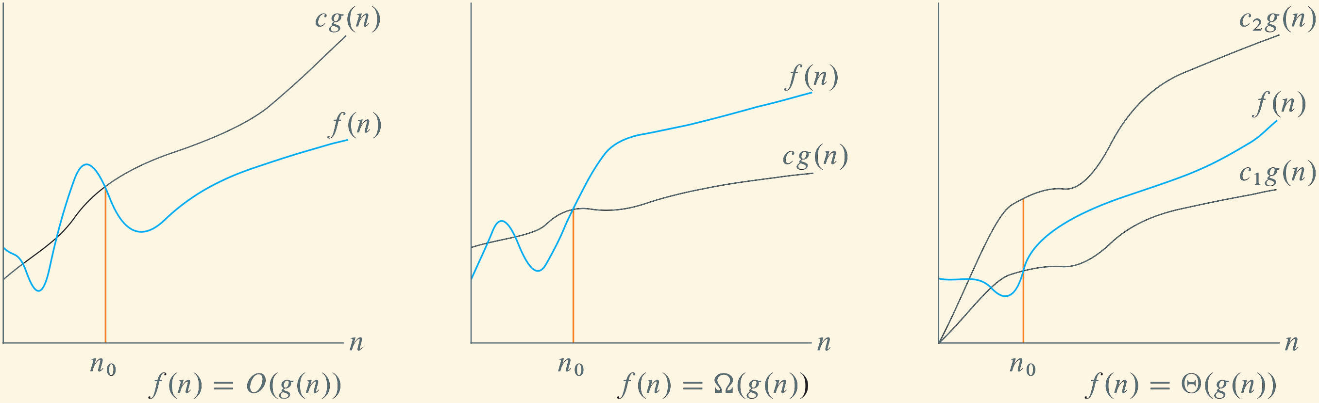
Recap: \(O\), \(\Omega\), and \(\Theta\) Notation
The lecture introduced asymptotic notation to describe the growth of a function \(f(n)\):
- \(\boldsymbol{O(g(n))}\): upper bound (grows no faster than)
- \(\boldsymbol{\Omega(g(n))}\): lower bound (grows at least as fast as)
- \(\boldsymbol{\Theta(g(n))}\): tight bound (same order of growth)
The picture below summarizes the idea: for sufficiently large \(n\), \(f(n)\) is above, below, or between multiples of \(g(n)\).
Multiple-Choice Questions
Multiple-Choice Questions
On the xSITe course page, navigate to Assessments → Quizzes → Week 02 Lab Exercise 1: Multiple Choice Questions — Running Times of Algorithms.
Select the best answer for each of the following four questions. You may refer to your notes or the lecture slides.
Exercise 1: Question 1
Suppose an algorithm allocates an array \(a\) of length \(n\), where each element is a 32-bit integer. The algorithm computes the following sum using a nested loop:
\[ S = \sum_{i=0}^{n-1}\sum_{j=0}^{n-1} a[i] \cdot a[j] \]
Which statement best aligns with the standard definition of basic steps in asymptotic analysis?
- Each multiplication \(a[i] \cdot a[j]\) is a basic step only when \(i = j\).
- Each multiplication \(a[i] \cdot a[j]\) is not a basic step because there are \(n^2\) total multiplications.
- Each multiplication \(a[i] \cdot a[j]\) is a basic step because both operands are fixed-width 32-bit integers.
- Whether \(a[i] \cdot a[j]\) is a basic step depends on whether \(n\) is a power of 2.
Exercise 1: Question 2
Consider the following pseudocode, where a is an array of length \(n\):
for i ← 0 .. n - 1 (both end points inclusive)
    if i > 0 then
        for j ← 0 .. i - 1
            a[i] ← i - j
Exactly how many times is the assignment to a[i] executed, as a function of \(n\)?
- \(n(n+1)/2\)
- \(n^2\)
- \(n(n-1)/2\)
- \(n\)
Exercise 1: Question 3
For sufficiently large \(n\), which ordering from slowest-growing to fastest-growing is correct?
\[\begin{align*} \text{a.}\quad & O(\log^2 n) &&\subset\quad O(\sqrt{n}) &&\subset\quad O(n) &&\subset\quad O(n\log n) \\ \text{b.}\quad & O(\log^2 n) &&\subset\quad O(n) &&\subset\quad O(\sqrt{n}) &&\subset\quad O(n\log n) \\ \text{c.}\quad & O(\sqrt{n}) &&\subset\quad O(\log^2 n) &&\subset\quad O(n) &&\subset\quad O(n\log n) \\ \text{d.}\quad & O(\log^2 n) &&\subset\quad O(\sqrt{n}) &&\subset\quad O(n\log n) &&\subset\quad O(n) \end{align*}\]
Exercise 1: Question 4
Use the Master Theorem to solve the recurrence \(T(n) = 3T(n/2) + n\). What is the asymptotic solution?
Master Theorem
Let \(a \ge 1\) and \(b > 1\) be constants, and let \(f(n)\) be a function with \(f(n) \ge 0\) for all sufficiently large \(n\). Consider recurrences of the form \(T(n) = a\,T\left(\frac{n}{b}\right) + f(n)\) for values of \(n\) for which the recurrence is defined (e.g., \(n=b^k\)). Let \(p = \log_b a\).
- If \(f(n) \in O\bigl(n^{p-\varepsilon}\bigr)\) for some \(\varepsilon > 0\), then \(T(n) \in \Theta\bigl(n^p\bigr)\).
- If there exists \(k \ge 0\) such that \(f(n) \in \Theta\bigl(n^p \log^k n \bigr)\), then \(T(n) \in \Theta\bigl(n^p \log^{k+1} n\bigr)\).
- If \(f(n) \in \Omega\bigl(n^{p+\varepsilon}\bigr)\) for some \(\varepsilon > 0\) and there exist constants \(c < 1\) and \(n_0\) such that for all \(n \ge n_0\) we have \(a\,f\left(\frac{n}{b}\right) \le c\,f(n)\), then \(T(n) \in \Theta\bigl(f(n)\bigr)\).
a. \(\Theta(n^2)\quad\) b. \(\Theta(n)\quad\) c. \(\Theta(n \log n)\quad\) d. \(\Theta(n^{\log_2 3})\quad\)
Matrix Multiplication
Matrix Multiplication: Problem Statement
We study the running time of algorithms that multiply two square matrices.
Given two \(n\times n\) matrices \(\mathbf{A}\) and \(\mathbf{B}\), the product matrix \(\mathbf{C} = \mathbf{A}\cdot \mathbf{B}\) has elements defined by \[ C_{ij} = \sum_{k=0}^{n-1} A_{ik} B_{kj}. \]
Hence, each element \(C_{ij}\) is the dot product of \(\mathbf{A}\)’s \(i\)-th row with \(\mathbf{B}\)’s \(j\)-th column. Note that we adopt 0-based indexing.

Input Format for Matrices
You can test your code by providing input matrices from a text file with the following format:
- The first line contains a single integer \(n\), representing the number of rows/columns.
- The file then lists \(\mathbf{A}\), \(\mathbf{B}\), and \(\mathbf{C}_{\text{expected}} = \mathbf{A}\cdot\mathbf{B}\) (each \(n\) rows); numbers in a row are comma-separated.
- Blank lines are ignored, and
#starts a comment.
C++ Implementation Overview
Download the starter code from GitHub Pages. The ZIP archive contains a C++ project for the exercises on the following slides:
main_*.cpp- Entry points for programs that perform specific tasks, such as correctness checks and benchmarking
matrix_utilities.cppandmatrix_utilities.h- Matrix types and helper functions (including input parsing)
matmul_*.cppandmatmul_*.h- Stubs for matrix-multiplication algorithms
vega_lite_plot.cppandvega_lite_plot.h- Utilities for plotting
makefile-
File to compile the project using
make
Understanding the Matrix Type
The starter code defines the matrix type in matrix_utilities.h:
MatrixInt64is a type alias for a 2D vector of 64-bit signed integers.Access element \((i, j)\) as
matrix[i][j].Create an \(n \times n\) zero matrix:
Why int64_t? When multiplying large matrices, intermediate sums can overflow 32-bit integers (even when the input entries fit in 32-bit). Using 64-bit integers provides a safety margin.
Triple Loop
Exercise 2a: Triple-Loop Matrix Multiplication
Recall the definition of matrix multiplication: \(C_{ij} = \sum_{k=0}^{n-1} A_{ik} B_{kj}.\) Your task is to implement this summation as a triple loop over \(i\), \(j\), and \(k\) (in this order). In the provided ZIP archive, complete the function stub matmulIJK() in matmul_ijk.cpp.
To compile and test locally, run the following commands:
Upload your solution to Gradescope. Detailed instructions are provided on xSITe (Dropbox \(\rightarrow\) Week 02 Lab Exercise 2a: Gradescope—Triple-Loop Matrix Multiplication).
Divide and Conquer
8-Fold Block-Recursive Matrix Multiplication: Key Idea
Block-recursive matrix multiplication is a divide-and-conquer algorithm that multiplies matrices by splitting them into equally-sized quadrants:
\[\begin{equation*} \mathbf{A}= \begin{pmatrix} \mathbf{A}_{11} & \mathbf{A}_{12}\\ \mathbf{A}_{21} & \mathbf{A}_{22} \end{pmatrix},\quad \mathbf{B}= \begin{pmatrix} \mathbf{B}_{11} & \mathbf{B}_{12}\\ \mathbf{B}_{21} & \mathbf{B}_{22} \end{pmatrix},\quad \mathbf{C}= \begin{pmatrix} \mathbf{C}_{11} & \mathbf{C}_{12}\\ \mathbf{C}_{21} & \mathbf{C}_{22} \end{pmatrix}. \end{equation*}\]
Then compute the four blocks of \(\mathbf{C}\) using 8 smaller multiplications (plus 4 additions):
\[\begin{equation*} \begin{aligned} \mathbf{C}_{11} &= \mathbf{A}_{11}\mathbf{B}_{11} + \mathbf{A}_{12}\mathbf{B}_{21}\\ \mathbf{C}_{12} &= \mathbf{A}_{11}\mathbf{B}_{12} + \mathbf{A}_{12}\mathbf{B}_{22}\\ \mathbf{C}_{21} &= \mathbf{A}_{21}\mathbf{B}_{11} + \mathbf{A}_{22}\mathbf{B}_{21}\\ \mathbf{C}_{22} &= \mathbf{A}_{21}\mathbf{B}_{12} + \mathbf{A}_{22}\mathbf{B}_{22}\\ \end{aligned} \end{equation*}\]
Divide and Conquer: Why Power-of-2 Sizes?
The recursive algorithm splits matrices into equal quadrants. This procedure requires the matrix dimension to be divisible by 2 at each level of recursion.
Problem: If \(n\) is not a power of 2 (e.g., \(n=3\)), we cannot split evenly all the way down to \(1 \times 1\) submatrices.
As the following slide explains, we solve this issue by padding the input matrices with zeros if necessary.
Divide and Conquer: Padding
- Find the smallest power of 2 that is \(\ge n\). The C++ code calls this number
padded_dim. For example, if \(n=3\), thenpadded_dim = 4. - Embed \(\mathbf{A}\) and \(\mathbf{B}\) in
padded_dim-by-padded_dimmatrices, filling extra elements with zeros. - Multiply the padded matrices using the recursive algorithm.
- Extract the top-left \(n \times n\) block of the result.

Why Padding Preserves Correctness
Consider the product \(C_{ij} = \sum_{k=0}^{n-1} A_{ik} B_{kj}\).
When we pad \(\mathbf{A}\) and \(\mathbf{B}\) with zeros to size padded_dim \(> n\):
- For \(\boldsymbol{i, j < n}\):
The extra terms in the sum (where \(k \ge n\)) are \(A_{ik} \cdot B_{kj} = 0 \cdot B_{kj} = 0\). The result is unchanged. - For \(\boldsymbol{i \ge n}\) or \(\boldsymbol{j \ge n}\):
These elements of \(\mathbf{C}\) are zeros. We discard them.
Conclusion: The top-left \(n \times n\) block of the padded product equals the true product \(\mathbf{A} \cdot \mathbf{B}\) of the unpadded matrices.
What You Need to Implement
If you haven’t already, download the starter files.
The starter code provides matmulDivideConquer8(), a wrapper function with padding logic already implemented.
Your task: Implement the recursive helper function blockMatmulAdd() that:
- Handles the base case (\(1 \times 1\) submatrix).
- Computes the 8 recursive calls for the four quadrants of \(\mathbf{C}\):
- \(\mathbf{C}_{11} \mathrel{+}= \mathbf{A}_{11}\mathbf{B}_{11}\), then \(\mathbf{C}_{11} \mathrel{+}= \mathbf{A}_{12}\mathbf{B}_{21}\)
- Similarly for \(\mathbf{C}_{12}\), \(\mathbf{C}_{21}\), \(\mathbf{C}_{22}\)
Exercise 2b: 8-Fold Block-Recursive Matrix Multiplication
To implement matrix multiplication recursively, complete the recursive helper function blockMatmulAdd() in matmul_divide_conquer.cpp, provided in the ZIP archive. The wrapper matmulDivideConquer8(), including padding and input checks, is already implemented.
Implementation trick: Do not copy \(A_{11},A_{12},\dots\) into new matrices. Instead, treat each submatrix as a view into the entire \(n\times n\) matrix: represent it by (row_offset, col_offset, size) and access elements via index offsets.
To compile and test locally, run the following commands:
Upload your solution to Gradescope. Detailed instructions are provided on xSITe (Dropbox \(\rightarrow\) Week 02 Lab Exercise 2b: Gradescope—8-Fold Block-Recursive Matrix Multiplication).
Benchmarking
From Theory to Measurement
Asymptotic notation tells us how an algorithm’s running time grows as the input size \(n\) increases. However, wall-clock time also matters: two \(\Theta(n^3)\) algorithms can differ by a large constant factor, which can significantly affect real-world performance.
In the following exercise, you will measure execution time on your computer. You do not need to write timing code yourself: a provided program runs the algorithms, measures the time, and produces a table and a plot.
Your task is to interpret the results:
- Look for the overall trend as \(n\) increases.
- Notice that constant factors and overhead can matter in practice.
Small fluctuations from run to run are normal; focus on the pattern.
Exercise 2c: Benchmarking and Analysis
Compile and run the provided benchmarking program to measure the running times of both matrix multiplication algorithms for various matrix sizes \(n\):
The optional argument max_n specifies the largest matrix dimension to benchmark (must be a power of 2, at least 8). The default is 64. For example, ./benchmark 256 tests sizes 8, 16, 32, 64, 128, and 256. The program will output a table of running times and generate a plot.
Your task: Submit a short report (PDF or DOCX) that includes:
- The generated plot showing running time versus \(n\) for both algorithms.
- The theoretically expected running times for each algorithm, with justification.
- A discussion of whether the measurements support the theoretical predictions.
- Upload your report to xSITe (Dropbox \(\rightarrow\) Week 02 Lab Exercise 2c: Benchmarking and Analysis).
Conclusion
Summary of Key Learning Outcomes
- Used \(O\)/\(\Omega\)/\(\Theta\) notation and the Master Theorem to classify the growth rates of divide-and-conquer recurrences. ↪
- Built a working block-recursive matrix multiplication by expressing subproblems via offsets, decomposing into quadrants, and handling the base case correctly. ↪
- Interpreted empirical performance differences between algorithms with the same \(\Theta(n^3)\) scaling, attributing gaps to constant factors (e.g., call overhead and compiler behavior). ↪
- Connected theory to data by benchmarking, checking scaling trends (e.g., when doubling \(n\)), and assessing whether the measurements align with the predicted asymptotics. ↪
Outlook
Challenges to explore on your own:
- Change the loop from \(i\)-\(j\)-\(k\) to \(i\)-\(k\)-\(j\). Faster or slower? Why?
- Replace 8-fold recursion with Strassen’s 7-fold recursion for \(\Theta(n^{2.81})\). See Section 4.2 of Cormen et al. (2022).
Next week’s topics:
This lab explored divide-and-conquer strategies and asymptotic analysis through matrix multiplication. Next week continues these themes with two classic sorting algorithms.
- Quicksort: A divide-and-conquer sorting algorithm—more practice analysing recurrences.
- Heapsort: Introduces heaps, a data structure that efficiently maintains a collection when elements are inserted or removed.
Bibliography
Week 02: Running Times (Lab)