Week 01: Foundations (Lecture)

Michael T. Gastner

2026-01-05

Intro

Learning Objectives

By the end of this lecture, you should be able to:

1. Define the terms data structure and algorithm.
2. Explain why studying data structures and algorithms is important.
3. Identify the key properties and use cases of arrays, a baseline data structure.
4. Use C++ vectors to create and manage dynamic arrays.
5. Verbally describe the insertion-sort algorithm for sorting an array.
6. Verify the correctness of the insertion-sort algorithm through logical reasoning and test cases.
7. Implement the insertion-sort algorithm in C++.
8. Compile and execute a C++ program using a makefile.

What is a Data Structure?

Definition

A data structure is a method of storing and organizing data to enable efficient access, manipulation, and modification.

Examples:

• An array stores elements in contiguous memory locations and supports constant-time access by index.
• A linked list consists of nodes that contain data and pointers to the next (and possibly previous) node, allowing for efficient insertions and deletions given a pointer to the node.

What is an Algorithm?

Choosing suitable data structures is a key aspect of designing efficient and scalable algorithms.

Definition

An algorithm is a well-defined computational procedure that accepts input values and produces output values in a finite amount of time.

Examples:

• Insertion sort and merge sort sort a sequence into ascending order.
• Binary search finds a target value in a sorted array.
• Dijkstra’s algorithm finds shortest paths in a weighted graph, such as a transportation network.

Why Data Structures and Algorithms Matter

Studying data structures and algorithms helps you design usable software. In this course, we will repeatedly ask these practical questions about computational procedures:

• Is it correct?

• Does it always terminate?

• Given a particular data structure as input, how much

  • time does the procedure take?
  • memory does the procedure use?

Arrays

Arrays: the Baseline Data Structure

An array is the simplest data structure, designed to store a collection of elements.

• Each element occupies the same number of bytes in memory.
• Each element is identified by a numeric index.
• Elements are stored in contiguous memory locations.

Arrays: Key Properties

Memory Layout

Suppose the array begins at memory address \(a\), and each element requires \(b\) bytes of memory:

• Indexing from 1: The \(i\)-th element occupies memory from \(a + b(i - 1)\) to \(a + b\,i - 1.\)
• Indexing from 0: The \(i\)-th element occupies memory from \(a + b\,i\) to \(a + b(i + 1) - 1.\)

The “\(-1\)” appears because the byte range is inclusive.

Access Time

We adopt the RAM model: the time required to access an array element by index is independent of the index.

Dynamic Arrays in Practice: C++ vector

In C++, the Standard Template Library provides std::vector, a dynamic array type.

Key properties:

• Stores elements in contiguous memory locations (like an array).
• Supports constant-time access by index: v[i].
• Can grow and shrink at runtime:
  • push_back(x) appends an element.
  • pop_back() removes the last element.
• Tracks its current number of elements with v.size().

A vector is the default choice when you need an “array whose size can change.”

Evidence of Contiguity: Addresses of Vector Elements

We can verify contiguity by printing the addresses of the elements:

• If the elements are stored contiguously, the addresses of v[i] and v[i+1] differ by the element size.
• For example, if v is a vector<int> and sizeof(int) = 4, then the addresses should increase by 4 bytes.

You can download a demo program by unzipping this ZIP file, where we print:

• the values v[i]
• the addresses &v[i]

The purpose of this program is to observe that the addresses form a regular pattern: each element starts immediately after the previous one. The content, build process, and output from the program are shown below.

Dynamic Arrays in Practice: C++ vector

In the code below:

• We cast &v[i] to const void* so that streaming it to std::cout prints the pointer value (the address) rather than treating it as character data.
• std::ptrdiff_t is the signed integer type used to store the result of subtracting two pointers (i.e., the offset between two addresses):

#include <cstddef>
#include <iostream>
#include <vector>

int main() {
  const std::vector<int> v{42, -17, 9382, 0, 30};
  std::cout << "sizeof(int) = " << sizeof(int) << " bytes\n";
  for (std::size_t i = 0; i < v.size(); ++i) {
    std::cout << "v[" << i << "] is at " << static_cast<const void *>(&v[i]);
    if (i > 0) {
      const std::ptrdiff_t d = &v[i] - &v[i - 1];
      std::cout << "  (diff=" << d * sizeof(int) << " bytes)";
    }
    std::cout << "\n";
  }
}

Compile and Run the Demo Program

Navigate to the directory containing the demo program and enter the following commands in a Terminal:

#| label: compile_run_vector_addresses
#| echo: true
#| eval: true
cd exercise_code/vector_addresses
rm -f vector_addresses
g++ -std=c++20 vector_addresses.cpp -o vector_addresses
./vector_addresses

All address differences in the output shown on the previous slide are equal to sizeof(int). Consequently, the memory addresses for the elements of v are contiguous.

Task: Replace int with other data types and convince yourself that elements of non-integer vectors also occupy contiguous blocks of memory.

Insertion Sort

Application of Arrays: Insertion Sort

Sorting rearranges the elements of an array into nondecreasing order. The elements to be sorted are referred to as keys. In this section, we study the classic insertion sort algorithm.

Sorting Problem

Input: Sequence of numbers \(\langle a_1, a_2, \ldots, a_n\rangle\)

Output: Permutation \(\langle a_1', a_2', \ldots, a_n'\rangle\) such that \(a_1' \leq a_2' \leq \ldots \leq a_n'.\)

Example

Input: \(\langle 31, 41, 59, 26, 41, 58\rangle\)

Output: \(\langle 26, 31, 41, 41, 58, 59\rangle\)

Insertion Sort: Core Idea

Generated with the help of OpenArt.

Imagine sorting a deck of cards. At all times, the cards in your hands remain sorted, and they are exactly the cards you have picked up so far.

The next slide formalizes this idea.

Insertion Sort in Words

1. Start with empty hands and a pile of cards on the table.

2. Pick one card, say \(X\), from the pile.

3. Insert \(X\) into the correct position among the sorted cards in your hands:

   1. Compare \(X\) with the cards in your hands from right to left.
   2. When you find a card \(Y\) with a value \(\le X\), place \(X\) immediately to the right of \(Y.\)
   3. If no such \(Y\) exists, place \(X\) in the leftmost position.

4. Repeat steps 2–3 until all cards are in your hands.

Video Tutorial: Insertion Sort

Here is a video tutorial on insertion sort. You can use YouTube’s playback features to view closed captions.

Note that the video uses 1-based indexing for arrays—as does our textbook (Cormen et al., 2022)—whereas C++ uses 0-based indexing.

Exercises at the End of the Video

Solution for Exercise 1 at the End of the Video

Solution for Exercise 2 at the End of the Video

Solution for Exercise 3 at the End of the Video

Check Your Exercise Solutions in the Insertion-Sort App

Open the app: https://apps.michael-gastner.com/insertion-sort/.

Stepping Through the Algorithm: Playback + Array State

Use the buttons to watch the array being sorted.

Important Variables in Insertion Sort

• active_key (shown in light blue): the value currently being inserted into the sorted left subarray
• i: number of keys sorted so far (sorted left subarray is a[0 .. i - 1]; 0-based indexing)
• h: index of the hole—the empty slot left behind after taking out active_key; it moves left as larger elements are shifted right, and active_key is eventually placed at a[h]

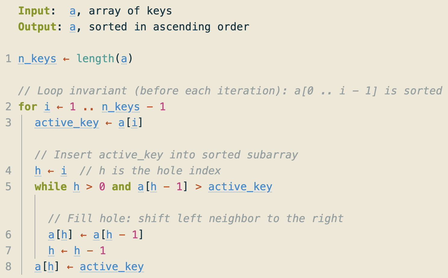
Insertion Sort: Pseudocode (As Used in the App)

Below the Array State panel, the app displays pseudocode with these features:

• 0-based indexing (as in C++).
• As you step through the algorithm, the current line is highlighted.
• Hover over a variable name (blue) to see its current value.

Figure 1: Pseudocode displayed at https://apps.michael-gastner.com/insertion-sort/.

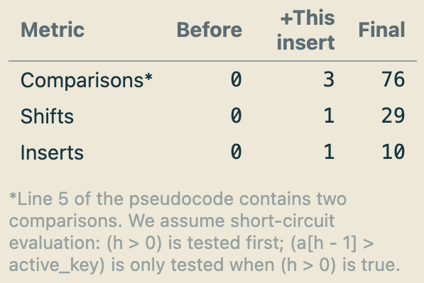
Insertion-Sort App: Statistics Panel

To the right of the pseudocode, the app displays a Statistics panel that counts work done as you step through the algorithm:

• The columns Before, +This insert, and Final show the totals before the current outer loop, what this iteration adds, and the running total.
• Hover over a metric to highlight the corresponding line(s) in the pseudocode.

We will connect these counts to running time in the next lecture.

Just Checking: Interpreting Insertion-Sort Statistics

During one outer iteration (i.e., one insertion), insertion sort performed 7 comparisons and 3 shifts.

Recall: the while condition is h > 0 and a[h - 1] > active_key, and comparisons are counted with short-circuit evaluation. What must be true?

1. The array contained duplicate keys, and a tie occurred in this iteration.
2. The initial index of active_key was equal to the index after the insertion.
3. active_key was inserted at index 0.
4. active_key was inserted at index 4.

Insertion Sort: The Loop Invariant

Definition

A loop invariant is a property \(\boldsymbol{I}\) that we require to hold at the loop head (i.e., right before the loop condition is checked). It may be false inside the loop body.

A well-chosen loop invariant is a proof tool. Its value at termination can reveal whether an algorithm is correct for any valid input.

Loop invariant of insertion sort: At the start of each for loop iteration i in line 2 of the pseudocode in Figure 1, the subarray a[0 .. i - 1] is sorted.

How We Use a Loop Invariant

To prove correctness, we must show:

1. Initialization: Property \(I\) holds the first time execution reaches the loop head.
2. Preservation: If \(I\) holds at the loop head and the loop condition is true, then after executing one iteration, \(I\) holds again at the next visit to the loop head.
3. Termination: The loop eventually stops.
4. Exit ⇒ Goal: When the loop stops, \(I\) together with the fact that the loop condition is false implies the postcondition (the algorithm’s goal).

Correctness of Insertion Sort (Proof Sketch)

Goal: When the algorithm finishes, a[0 .. n_keys - 1] is sorted.

Outer-loop invariant (at the loop head): At the start of each outer iteration with index i (1 ≤ i ≤ n_keys - 1), the subarray a[0 .. i - 1] is sorted.

1. Initialization: The first iteration has i = 1, so a[0 .. 0] has one element and is trivially sorted.
2. Preservation: Assuming a[0 .. i - 1] is sorted, the loop body inserts active_key = a[i] into its correct position because of the while loop condition a[h - 1] > active_key on line 5 of Figure 1. Thus, a[0 .. i] sorted.
3. Termination: The outer loop runs over the finite range i = 1 .. n_keys - 1, so it is guaranteed to terminate. In the while loop, h decreases by 1 on each shift and is bounded below by 0, so the while loop must also terminate.
4. Exit ⇒ Goal: After the last iteration, the invariant ensures that a[0 .. n_keys - 1] is sorted.

Insertion Sort in C++

Insertion Sort in C++

Let us move from theory to practice and implement insertion sort in C++. Download this ZIP file, which splits the project into these files, following common C++ practices:

• Header files (.h) contain function declarations.
• Source files (.cpp) contain function definitions (the function bodies).

For example, insertion_sort.h declares insertionSort(...), while insertion_sort.cpp defines it.

insertion_sort.h

#ifndef INSERTION_SORT_H
#define INSERTION_SORT_H

#include <vector>

void insertionSort(std::vector<int> &a);

#endif  // INSERTION_SORT_H

The preprocessor directives at the top and bottom implement an include guard, which prevents multiple inclusions of the same header file.

insertion_sort.cpp

#include "insertion_sort.h"

#include <cstddef>
#include <vector>

void insertionSort(std::vector<int> &a) {
  for (std::size_t i = 1; i < a.size(); ++i) {
    const int active_key = a[i];
    std::size_t h = i;
    while (h > 0 && a[h - 1] > active_key) {
      a[h] = a[h - 1];
      --h;
    }
    a[h] = active_key;
  }
}

Makefile to Build the C++ Program

In the labs, you will write C++ code and submit your programs to Gradescope for autograding. Gradescope requires a makefile so that the autograder can compile your submission consistently.

We will always provide the required makefile, so you do not need to write one yourself. However, you do need to know how to use a makefile to compile and run your C++ programs locally before submitting them to Gradescope.

The following slides explain how to accomplish this task.

Compiling the C++ Program

Place the makefile alongside all required .cpp and .h files in the same directory. Then compile the code as follows:

1. Run make clean to remove build artifacts from previous compilations. This step avoids confusing results if you have an old executable or stale object files.
2. Run make to build the program.

#| label: build_cpp_insertion_sort
#| echo: true
#| output: false
#| eval: true
cd exercise_code/insertion_sort
make clean
make

If compilation succeeds, you will obtain an executable (as specified by TARGET in the makefile). In this example, the executable is named insertion_sort.

Running the Insertion Sort C++ Program

The ZIP file you downloaded contains sample input files named test_0.txt:

30, -6, 0, 5, -2, 8, -7, 3, 1, -4, 6

Then run:

#| label: run_cpp_insertion_sort
#| echo: true
#| eval: true
cd exercise_code/insertion_sort
make run FILE=test_0.txt

The program prints the sorted integers separated by commas.

Testing Insertion Sort C++ Code Using Gradescope

For lab assignments, you will submit your C++ code to Gradescope, which will automatically test your code. Let’s use insertion_sort.cpp as an example.

Navigate to the assignment “Week 01 Lecture: Gradescope Demo—Insertion Sort” in the xSITe Dropbox for our course. This assignment is for demonstration purposes only and won’t be graded. However, please read the assignment instructions carefully because the lab assignments will be similar.

Follow the link to Gradescope and upload the file insertion_sort.cpp. Once submitted, the Gradescope autograder will run the tests and provide feedback on your code.

Conclusion

Summary of Key Learning Outcomes

1. You can define data structures. ↪
2. … and algorithms. ↪
3. … and explain why studying data structures and algorithms matters. ↪
4. You explored arrays, a fundamental data structure that stores elements in contiguous memory locations. ↪
5. … and their C++ implementation: vectors, which can be dynamically resized at runtime. ↪
6. You examined an important application of arrays: sorting, focusing on the insertion sort algorithm. ↪
7. You analyzed the correctness of insertion sort by applying a loop invariant. ↪
8. You implemented insertion sort in C++ as a multi-file project (header + source files). ↪
9. … and used a makefile to compile and run it. ↪

Outlook

In the lab later this week, you will study an alternative sorting algorithm called merge sort. Here is a preview:

Bibliography

Cormen, T.H. et al. (2022) Introduction to algorithms. 4th ed. MIT Press.