Week 01: Foundations (Lab)
2026-01-08
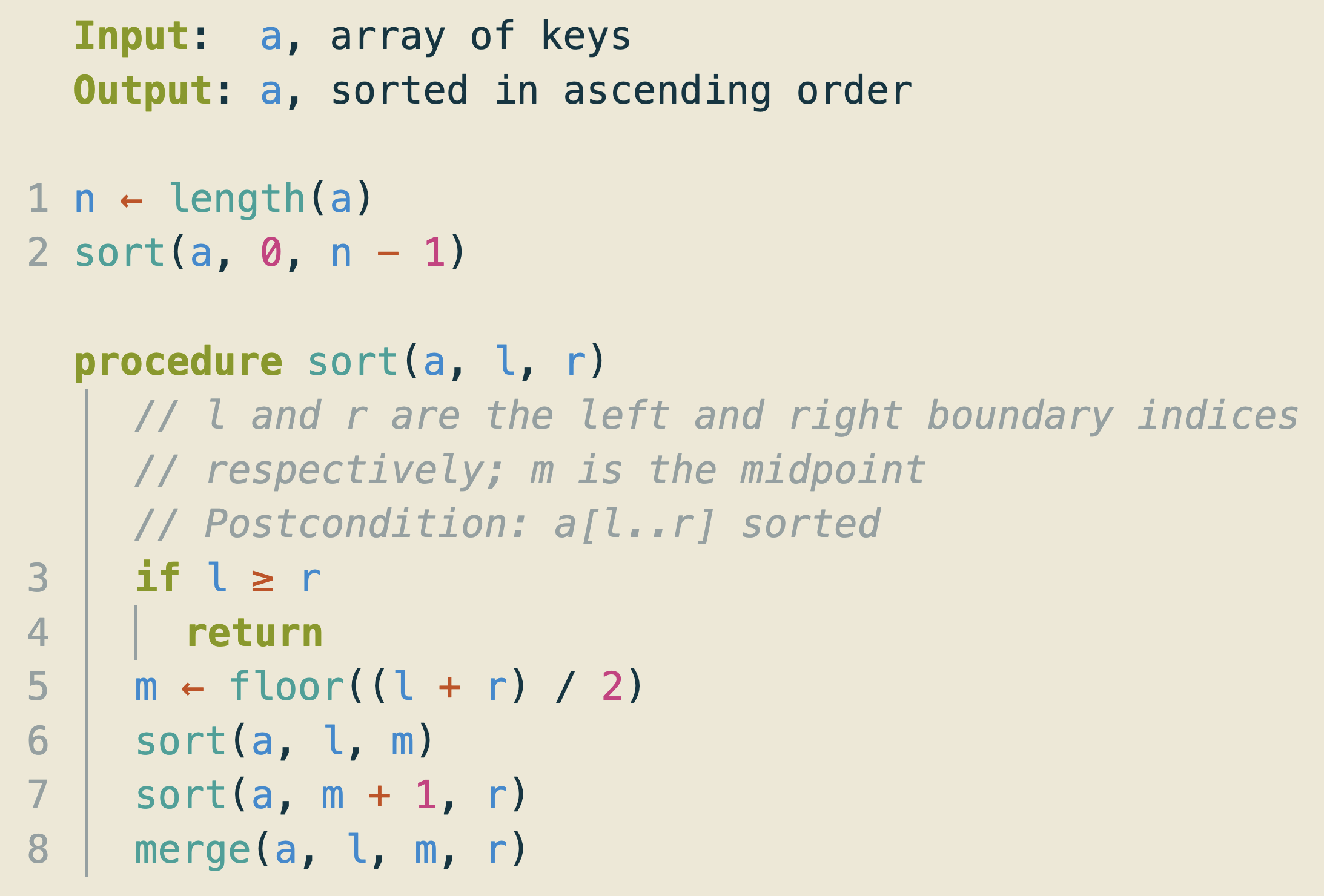
Pseudocode for Merge Sort
Note that the video and our textbook Cormen et al. (2022) adopt 1-based indexing. Here is the pseudocode for merge sort for 0-based indexing, as used by https://apps.michael-gastner.com/merge-sort/:
Example: Merge Sort Applied to an Array
The example on the right illustrates the merge sort algorithm applied to a numeric array, modeled after Figure 2.4 in Cormen et al. (2022).
Italicized numbers indicate the sequence in which the sort() and merge() procedures are invoked, starting with the initial call to sort(a, 0, 7).

Exercise 1: Merge Sort—Fill in the Gaps
Download the image on the right from GitHub Pages in PNG or PDF format. Adopting the pattern from the example on the previous page, complete the following tasks:
- Label the arrows with numbers indicating the sequence of the
sort()andmerge()procedure calls. - Fill in the correct values in the empty boxes.
You may use any drawing tool, such as Annotely. When finished, upload the completed image (e.g., as a screenshot) to xSITe (Dropbox → Week 01 Lab Exercise 1: Merge Sort—Fill in the Gaps).

Exercise 3a: Recursive Insertion Sort—Pseudocode
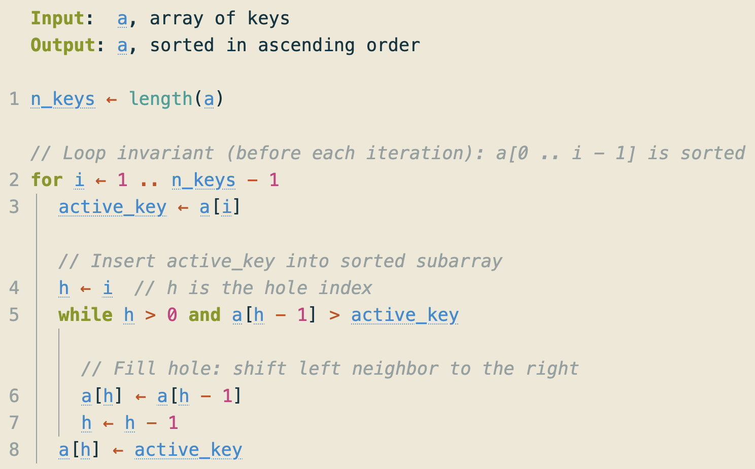
The lecture introduced insertion sort as the non-recursive algorithm shown below.
However, insertion sort can also be implemented as a recursive algorithm. To sort a[0..n], recursively sort the subarray a[0..(n-1)] and then insert a[n] into the sorted subarray. Write pseudocode for this recursive version. Submit your solution (e.g., a photo of your handwritten notes) to xSITe (Dropbox \(\rightarrow\) Pseudocode of Recursive Insertion Sort).
Plot of Running Time versus Array Size
